Real-World Efficiency: Tail-Specific Models vs. OEM Assumptions

Over time the performance of the aircraft may change quite a bit. Deterioration or installation of custom / minor modifications may not only result in the change in fuel burn that can be accounted for with performance factors but also modify the characteristics (shape of the curve) of the fuel consumption and consequently combined cost of fuel and time – Direct Operating Cost (DOC). This often causes the shift in where the true optimum speed lies, and cause OEM models to miss on a lot of potential savings.

Figure 1. Changes to the cost characteristics of mid-range aircraft over time (OEM vs QAR).¹

In the market a common misconception of tail-specific models appears, where providers refer to the application of performance factors as a modification to models themselves, causing confusion.

Let’s look at an example of how recommendations may differ for two aircraft tails in both of those cases. Assume both aircrafts have already flown for quite a while and may have some slight modifications.

First, after we apply the deterioration the the OEM performance models, we can obtain the characteristics curves that will be closer to the level of current aircraft fuel burn, but the recommended speeds will remain the same. While the average fuel burn will be adjusted to each aircraft, the underlying model will NOT be tail-specific.

Figure 2. Changes to the cost characteristics of the two mid-range aircrafts over time (OEM + APM Performance Factors).¹

In the second example, when we refer to our QAR-based Performance Models, we can see that when the models fit specifically to each tail’s performance, the shape of the curve of each individual aircraft may slightly change. Those differences add up and are the source of many unrealized savings.

Figure 3. Changes to the cost characteristics of the two mid-range aircrafts over time (QAR-Based Models).¹

The tail-specific models have a significant advantage in the accuracy of the estimations. They can adjust to the specific characteristics of a given aircraft, taking into account its real performance. We can see that by looking at the aircraft’s QAR (Quick Access Recorder) data. We can perform predictions with OEM (adjusted for deterioration) and QAR-based tail-specific models and look at the distribution of errors they produce on a number of samples (how much do they diverge from real fuel consumption readings).

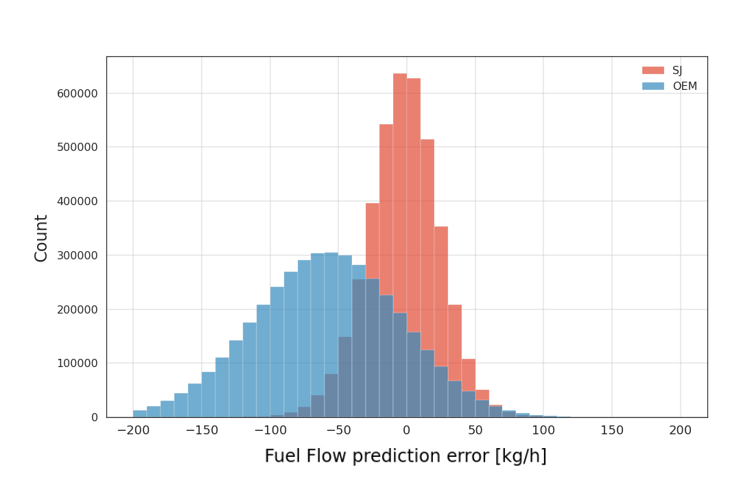
Figure 4. Distribution of fuel flow prediction error based on OEM (blue) and StorkJet (SJ) tail-specific performance models (red).

While the shift of the OEM distribution can be corrected with performance factors (you can imagine moving the blue bars to the right, to have a mean around the 0 value), the overall wideness of the distribution, resulting from the inaccuracies in the models, will not change significantly.

With that in mind, we’ve decided to take a closer look at what’s possible to achieve with OEM compared to our QAR-based, tail-specific performance models. We corrected the OEM models output for the deterioration and analysed the produced optima in the popular weather conditions.

Results

We have seen a savings between 0.1 up to 1% for a range of popular mid-range aircrafts in the most common weather and weight conditions. This difference may be even larger if your operations are unusual – noticeably colder/hotter weather, high weights, low company Cost Index or aircraft modifications applied.

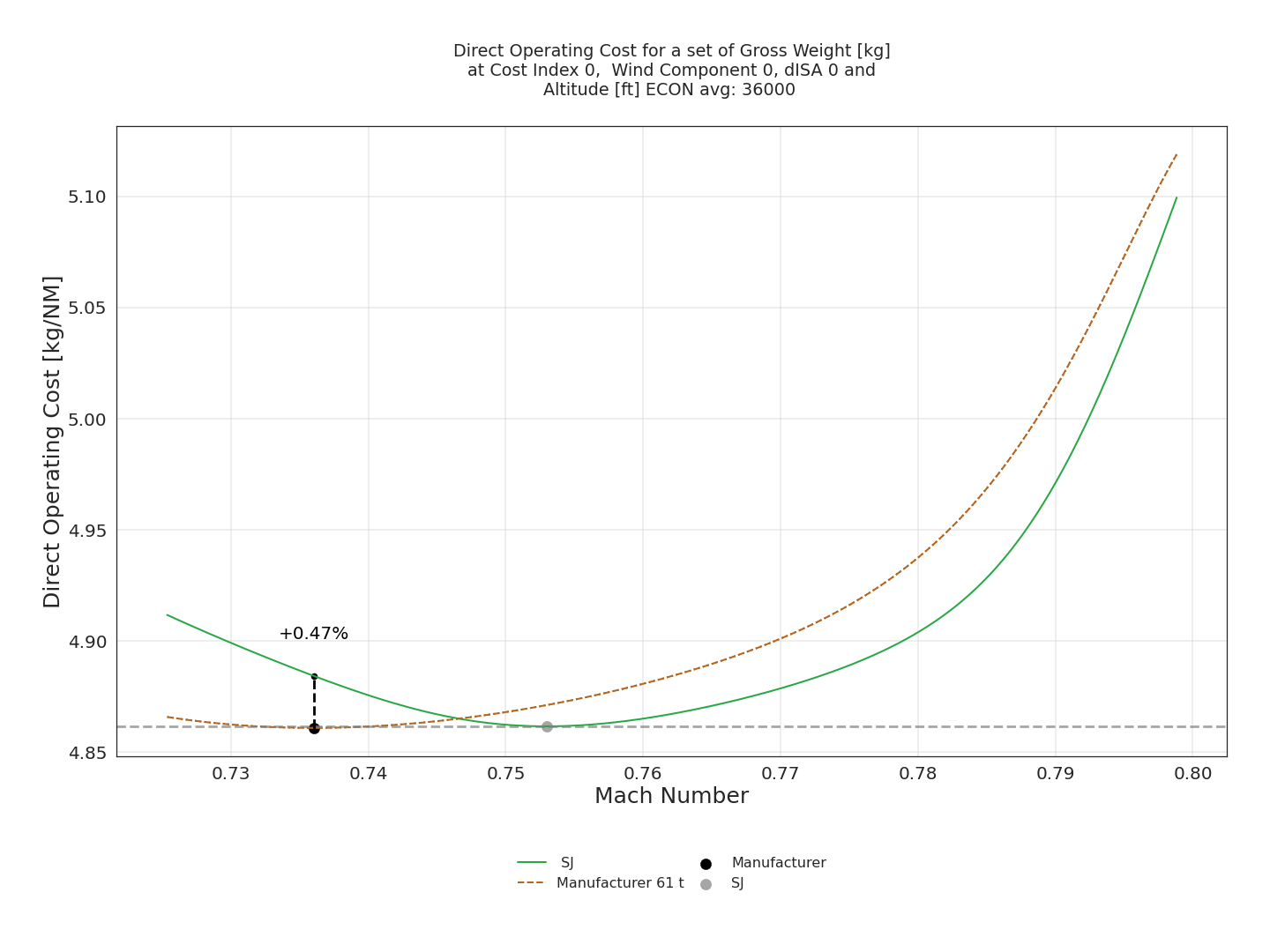
Figure 5. Example of mid-range aircraft OEM vs tail-specific models comparison.

In the example above we can notice that the optima produced by the manufacturer performance models will result in a recommendation that in reality will miss on 0.47% of cost savings.

To give a perspective, by selecting truly optimal speeds thanks to tail-specific models, on a fleet composed of mid range aircrafts, flying on average 2000 miles cruise segments in common conditions you may save from 10 up to 100 kg per flight depending on aircraft type. And as mentioned already those savings may be higher if you fly in non-standard conditions or with some aircraft modifications installed.

It’s worth noting that savings resulting from the application of the QAR driven performance model optimums diminish at a high Cost Index relative to Fuel Flow. For mid-range aircraft for CI > ~100, the importance of the time cost function becomes so high, that differences between performance models become negligible, while for the low Cost Indexes the time factor becomes less significant leading to the increase of potential savings.

¹Animations made with the help of Manim library.